Slides.knit

class: center, inverse, middle

.pull-left-wide {
  float: left;
  width: 66%;
}
.pull-right-wide {
  float: right;
  width: 66%;
}
.pull-right-wide ~ p {
  clear: both;
}

.pull-left-narrow {
  float: left;
  width: 30%;
}
.pull-right-narrow {
  float: right;
  width: 30%;
}

.pull-right-extra-narrow {
  float: right;
  width: 20%;
}

.pull-center {
  margin-left: 28%;
  width: 44%;
}

.pull-center-wide {
  margin-left: 17%;
  width: 66%;
}

.pull-center-medium {
  margin-left: 20%;
  width: 60%;
}

.pull-center-narrow {
  margin-left: 35%;
  width: 25%;
}

.tiny123 {
  font-size: 0.40em;
}

.small123 {
  font-size: 0.80em;
}

.large123 {
  font-size: 2em;
}

.red {
  color: red
}

.chaosred {
  color: #b33d3d
}

.orange {
  color: orange
}

.green {
  color: green
}

.blue {
  color: blue
}

/* Full-bleed plate slides: image fills the slide below the title */
.plate img {
  max-height: 390px;
  width: auto;
  max-width: 100%;
  display: block;
  margin: 0 auto;
}
.plate-tall img {
  max-height: 440px;
  width: auto;
  max-width: 100%;
  display: block;
  margin: 0 auto;
}
.plate-short img {
  max-height: 330px;
  width: auto;
  max-width: 100%;
  display: block;
  margin: 0 auto;
}
</style>

# Counting houses
## Mapping late medieval populations using the DOMUS* model

### **Christian Vedel**, University of Southern Denmark
### Chiara Zanardello, Toulouse School of Economics

### Email: [christian-vs@sam.sdu.dk](mailto:christian-vs@sam.sdu.dk)

### Updated 2026-09-16

#### **Density-based Object Mapping of Urban Structures*

---
name: intro

# Why count people who have been dead for 400 years?

.pull-left[
- **Population** counts is very rich information on economic development.
- **Malthusian link** to development: Output `$\Rightarrow$` Population.
- **City databases:** Bairoch et al. (1988); Bosker, Buringh & van Zanden (2013); **Buringh (2021)**: 2,258 cities, 700–2000. Relies heavily on inputations.
- **Applications:**
  - Nunn & Qian (2011): *potatoes raised urban population*
  - Bosker et al. (2013): *Europe–Middle East divergence*
  - Many more
- Worth adding new sources with ML tools.

]

.pull-right[
![Urban population](Figures/buringh_urban_population.png)
.small123[*All cities in Buringh (2021), summed.*]
]

.pull-right[
> .chaosred[**Very preliminary.**] A proof of concept. Ideas and applications are most welcome.
]

---
name: odense
class: plate

# A familiar place in 1593

.panelset[
.panel[.panel-name[1593]
![Odense 1593](Figures/odense_plain.jpg)
.small123[*Braun & Hogenberg, vol. V (1598), drawn 1593. Buringh (2021): 5,000 inhabitants in 1600 (1550 imputed).*]
]
.panel[.panel-name[What if we just count houses?]
![Odense 1593 with counted houses](Figures/odense_dots.jpg)
.small123[*Every dot is one structure: 883 houses, 36 towers, 33 defensive structures. The literature suggests the engravers were diligent (Van der Krogt 2008).*]
]
]

---
name: civitates

# The source: *Civitates Orbis Terrarum*

.pull-left[
.panelset[
.panel[.panel-name[Where it comes from]
- Edited in Cologne by **Georg Braun**; engraved and published by **Frans Hogenberg**. Six volumes, 1572–1617.
- **361 sheets, 543 views of 475 towns**; 95 pct. European. Over 50 towns appear more than once (Van der Krogt 2008).
- Drawings came from a wide network: Joris **Hoefnagel**'s travel sketches, Jacob **van Deventer**'s measured surveys, and copies of earlier prints.

.small123[
**Similar sources, readily available:** Münster, *Cosmographia* (1544–1628; hundreds of woodcut views) &middot; Van Deventer's manuscript plans (c. 1558–1575; ~226 towns) &middot; Blaeu, *Toonneel der Steden* (1649; 200+ Dutch plans) &middot; Merian, *Topographia* (1642–1654; ~2,100 views) &middot; Resen, *Atlas Danicus* (1677)
]
]
.panel[.panel-name[Can we trust it?]
- A **publishing enterprise, not a survey**: no sampling rule, no common scale. Selection followed contributors' travels and commercial appeal.
- Every plate passed through draftsmen, editors, and engravers. Monuments enlarged; repetitive housing schematised.
- But recognisability mattered: walls, churches, streets, and the overall fabric were what identified a town, and were kept (Nuti 1994; Ballon & Friedman 2007).
]
]
]

.pull-right[
![Civitates Orbis Terrarum](Figures/odense_colour.jpg)
.small123[*Odense coloured in a coloured map.*]
]

---
name: famous-cities
class: plate-short

# Some cities you might recognise

.panelset[
.panel[.panel-name[London]
![London](Figures/cities/london.jpg)
.small123[*Londinum Feracissimi Angliae Regni Metropolis, vol. I (1572). Old St Paul's still has the spire it lost in 1561: the drawing predates the print.*]
]
.panel[.panel-name[Paris]
![Paris](Figures/cities/paris.jpg)
.small123[*Lutetia vulgari nomine Paris, vol. I (1572).*]
]
.panel[.panel-name[Rome]
![Rome](Figures/cities/rome.jpg)
.small123[*Roma, vol. I (1572). The ancient walls enclose far more than the inhabited core.*]
]
.panel[.panel-name[Venice]
![Venice](Figures/cities/venice.jpg)
.small123[*Venetia, vol. I (1572).*]
]
.panel[.panel-name[Amsterdam]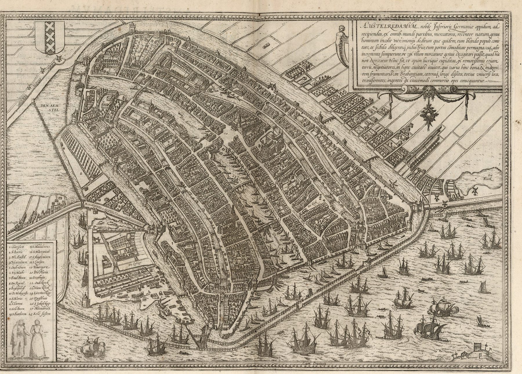
![Amsterdam](Figures/cities/amsterdam.jpg)
.small123[*Amstelredamum, vol. I (1572). Before the canal-ring expansion.*]
]
.panel[.panel-name[Istanbul]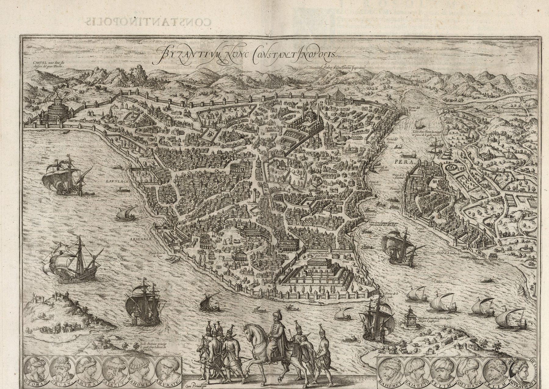
![Constantinople](Figures/cities/constantinople.jpg)
.small123[*Byzantium nunc Constantinopolis, vol. I (1572). The capital of the empire the atlas was meant to keep out.*]
]
.panel[.panel-name[Copenhagen]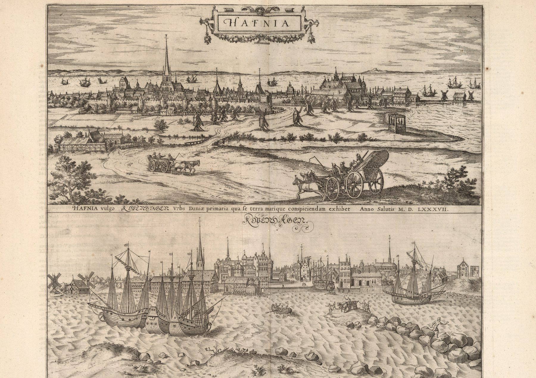
![Copenhagen](Figures/cities/copenhagen.jpg)
.small123[*Hafnia, vol. IV (1588). A profile view: the skyline is visible, the houses behind it are not.*]
]
.panel[.panel-name[Mexico & Cusco]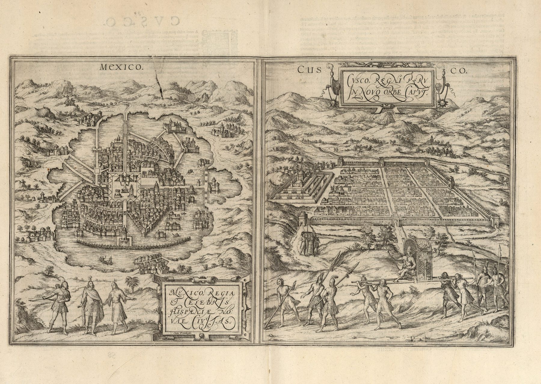
![Mexico and Cusco](Figures/cities/mexico.jpg)
.small123[*Mexico and Cusco, vol. I (1572). "Orbis Terrarum" was meant literally; 95 pct. of the towns are nevertheless European.*]
]
]

---
name: ottomans

# Why is there always a couple standing in the foreground?

.pull-left-wide[
- The Ottoman Empire was the military threat of the 16th century. A detailed bird's-eye view of a city's walls is also an intelligence document.
- Braun's answer, stated in the preface to volume I: put **people in local dress** on every plate.
- Islamic religious practice forbade images of humans, so *"the bloodthirsty Turk ... will never allow this book to be seen"*.
]

.pull-right-narrow[
![Figures on the Odense plate](Figures/odense_figures.jpg)
.small123[*Foreground figures on the Odense plate. The costumes were taken from contemporary costume books.*]
]

.pull-left-wide[
> Whatever we think of the argument, it tells us **how the makers saw the maps**: as accurate enough to be militarily useful.
]

---
name: what-to-extract
class: plate

# What can we extract from these maps?

.panelset[
.panel[.panel-name[Text]
.pull-left[
### Latin (title cartouche)
.small123[
*Civitatis episcopalis Othenarum sive Otthoniae, ut vulgo dicitur, Fioniae, insularum Daniae regni amoenissimae fertilissimaeque metropolis, secundum situm & figuram quam hoc seculo habet, delineatio. Anno partae per unicum mediatorem Christum salutis MDLXXXXIII. Genere, virtutibus, famaque illustri Henrico Ranzovio, imperiali et regio Danico consiliario, ducatuumque Slesvici, Holsatiae et Dithmarsiae gubernatore, summorum et optimorum conatuum promotore, impensas suppeditante.*
]
]

.pull-right[
### English
.small123[
*Depiction of the episcopal city of Othenarum, or Odense as it is commonly called, capital of Funen, the loveliest and most fertile of the islands of the Kingdom of Denmark, according to the situation and shape it has in this century. In the year of salvation, obtained through Christ our sole mediator, 1593. Heinrich Rantzau, illustrious by birth, virtue, and fame, counsellor to the Emperor and to the Danish King, governor of the duchies of Schleswig, Holstein, and Dithmarschen, and patron of the highest and best endeavours, bore the costs.*
]
]

.small123[
Braun's description on the verso adds: *"...distinguished by magnificent buildings and splendid churches, of which the noblest is the basilica of the King of Denmark, St Canute... The city has a large, wide market where tribunals are also held, and fish is sold."*
]
]

.panel[.panel-name[Type of building]
.pull-left-wide[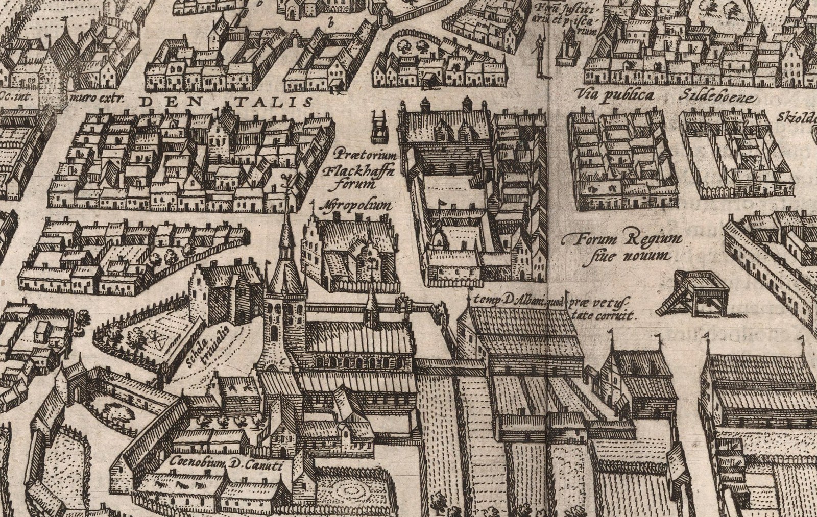
![Odense centre](Figures/odense_detail_centre.jpg)
]
.pull-right-narrow[
- **Churches:** *Coenobium D. Canuti*; *temp. D. Albani, quod prae vetustate corruit* (collapsed from age)
- **Civic:** *Praetorium* (town hall), *Forum Regium sive novum*, *Foru[m] Justitiarium et piscarium*
- **School:** *Schola trivialis*
- **Houses:** size, rows, gardens
]
]

.panel[.panel-name[Number of buildings]
.pull-left-wide[
![Odense with counted houses](Figures/odense_dots.jpg)
]
.pull-right-narrow[
### The simplest thing
- **Count the buildings.** One dot per visually separable structure.
- Ordinary houses, churches, towers, walls, large secular buildings, infrastructure.
- This is what we go for as a **proof of concept**.

.chaosred[*If only we could do this automatically...*]
]
]
]

---
class: inverse, middle, center

# Methods

---
name: methods-overview
class: middle

# DOMUS in one picture

.center[<img src="Figures/domus_pipeline.png" width="90%">]

.pull-center-wide[
.small123[*A plate goes in; a density map comes out. Its integral is the building count. Everything that follows is about how the model learns that map from a few thousand clicks.*]
]

---
name: cities-density
class: plate-short

# Revisiting our cities from before

.pull-left-wide[

.panelset[
.panel[.panel-name[London]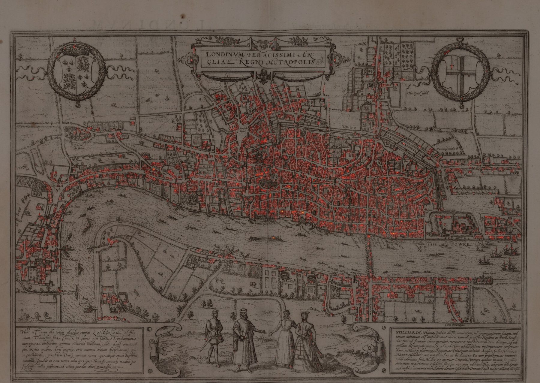
![London density](Figures/cities_density/london.jpg)
.small123[*Predicted density, class "ordinary building". Count: 2,933 houses.*]
]
.panel[.panel-name[Paris]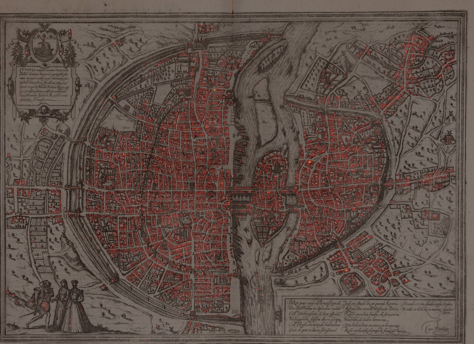
![Paris density](Figures/cities_density/paris.jpg)
.small123[*4,202 houses.*]
]
.panel[.panel-name[Rome]
![Rome density](Figures/cities_density/rome.jpg)
.small123[*1,681 houses. The empty land inside the ancient walls stays dark.*]
]
.panel[.panel-name[Venice]
![Venice density](Figures/cities_density/venice.jpg)
.small123[*1,865 houses.*]
]
.panel[.panel-name[Amsterdam]
![Amsterdam density](Figures/cities_density/amsterdam.jpg)
.small123[*3,262 houses.*]
]
.panel[.panel-name[Istanbul]
![Constantinople density](Figures/cities_density/constantinople.jpg)
.small123[*1,839 houses.*]
]
.panel[.panel-name[Copenhagen]
![Copenhagen density](Figures/cities_density/copenhagen.jpg)
.small123[*282 houses. A profile view: the model only sees the front row.*]
]
.panel[.panel-name[Mexico & Cusco]
.![Mexico & Cusco density](Figures/cities_density/mexico.jpg)
.small123[*627 houses across the two panels.*]
]
.panel[.panel-name[Odense]
![Odense density](Figures/cities_density/odense.jpg)
.small123[*883 houses.*]
]
]

]

.pull-right-narrow[
  > **Main idea**: We want to predict a heat map of where buildings are. A heat map which we can integrate to get the total building count.
]

---
name: back-of-envelope

# Back of the envelope

.pull-left-wide[
**Houses on the plate:** 883

**People per house:** 4.3
.small123[*(Leiden, 1561–1606; Van Steensel, van Oosten & Hooymans 2025)*]

`$$883 \times 4.3 \approx 3{,}800 \text{ inhabitants}$$`
]

.pull-right-narrow[
![Odense with counted houses](Figures/cities_density/odense.jpg)
]

--
.pull-left-wide[
  > *What do we get from other sources?*
> - 3000-3200 in 1570, 
> - 4000 in 1640.
> Source: [Christiensen [Trap] (2021)](https://trap.lex.dk/1536-1850_i_Odense_Kommune#-Befolkningsudvikling)
]

.pull-left[
- In practice our plan is to run a regression of the form
`$$Pop_i = \beta_0 + \beta_1 \cdot Houses_i + \varepsilon_i$$`
Or even
`$$log(Pop_i) = \beta_0 + \beta_1 log(Houses_i) + \varepsilon_i$$`
]

---
name: how

# How do we get the predictions?

.pull-left[
- We view this as a **density regression problem**: the model predicts a smooth map whose integral gives the building count.
- This approach allows us to handle overlapping and ambiguous structures effectively.
- If a human can identify *one* point from each building, then this is a sample from the underlying building density.

**Target:** each labelled point `$p_j$` becomes a Gaussian bump; the bumps are summed:

`$$d(u) = \sum_{j} \mathcal{G}_\sigma(u - p_j), \qquad \sum_u d(u) = N$$`

.small123[*Output grid u at 1/4 of input resolution; σ = 2 output pixels, kernel truncated at 3σ and normalised to sum to one.*]
]

.pull-right[
### Loss function

The network outputs a log-density `$z(u)$`; the density is `$\hat{d}(u) = e^{z(u)}$` and the count `$\hat{N} = \sum_u e^{z(u)}$`.

`$$\mathcal{L} = \underbrace{\frac{1}{|\mathcal{U}|}\sum_{u}\Big(e^{z(u)} - d(u)\,z(u)\Big)}_{\text{Poisson NLL:} \textbf{ where}} \;+\; \lambda\,\underbrace{\big|\hat{N} - N\big|}_{\textbf{how many}}$$`

- `$\lambda$` annealed from 10 to 0.1 over training: totals first, then localisation.

.small123[
**Why Poisson, not MSE?** Most pixels are zero; softplus + MSE collapses to all-zero output and the gradient dies. The Poisson gradient e<sup>z</sup> − d never vanishes where a building is.
]
]

---
name: methods-labelling
class: plate-tall

# Labelling and training: one click per building

.panelset[
.panel[.panel-name[Messina]
![Messina tile](Figures/labelled_tiles/12126102_Vol_I_49_Messana_Messina_x04608_y01536_dots.jpg)
.small123[*715 dots on one 1536 px tile. Blue = ordinary building, orange = religious, green = defensive, red = tower, purple = large secular, brown = infrastructure, pink = unclear.*]
]
.panel[.panel-name[Lyon]
![Lyon tile](Figures/labelled_tiles/12126024_Vol_I_10_Lugdunum_Lyon_x04608_y03840_dots.jpg)
.small123[*647 dots.*]
]
.panel[.panel-name[Douai]
![Douai tile](Figures/labelled_tiles/12126286_Vol_III_20_Douay_Douai_x04608_y02304_dots.jpg)
.small123[*785 dots. A Van Deventer-style plan: nearly everything is an ordinary building.*]
]
.panel[.panel-name[Leeuwarden]
![Leeuwarden tile](Figures/labelled_tiles/12126318_Vol_III_36_Leevwaerden_Leeuwarden_Franicker_Franeker_x03840_y03072_dots.jpg)
.small123[*541 dots.*]
]
.panel[.panel-name[Without dots]
![Messina tile plain](Figures/labelled_tiles/12126102_Vol_I_49_Messana_Messina_x04608_y01536_plain.jpg)
.small123[*The Messina tile as the coder sees it before clicking.*]
]
.panel[.panel-name[Numbers]
- **Codebook:** one dot on every visually separable structure, tagged with one of seven classes.
- **Two coders** (Chiara and me). Double-coded tiles are kept as two independent annotations.
- **So far:** ~10,700 dots on 118 tiles; 24 tiles from 29 held-out cities for testing.
- Tiles are cut from the plates on a fixed overlapping grid; the model trains and predicts on the same grid.
]
]

---
name: methods-density
class: plate

# What the model predicts: a density

.panelset[
.panel[.panel-name[Plate]
![Odense detail](Figures/odense_plain_detail.jpg)
.small123[*Odense, town centre.*]
]
.panel[.panel-name[Density]
![Odense density](Figures/odense_density_detail.jpg)
.small123[*Predicted density for the class "ordinary building". Red = mass. The integral over the plate is the count: 883.*]
]
.panel[.panel-name[Whole plate]
![Odense density full](Figures/odense_density.jpg)
.small123[*The same density over the full plate. Outlying farms and churches light up too.*]
]
]

---
name: methods-architectures

# Architectures

.pull-left[
### DOMUS-CNN
- **Encoder:** ResNet-18, ImageNet-pretrained, **frozen**.
- Feature pyramid at strides 4 / 8 / 16.
- **Decoder:** light U-Net; upsample and re-inject encoder features via skip connections (~0.5M trained parameters).
]

.pull-right[
### DOMUS-ViT
- **Encoder:** ViT-S/16 with self-supervised **DINO** weights, **frozen**.
- One feature map at stride 16, no pyramid.
- **Decoder:** plain upsampling back to stride 4, no skips (ViTDet-style).
]

.pull-left-wide[
> Both output a density map for each building type we label.
]

---
name: training

# Training

.pull-left[
- **Data:** 105 labelled tiles for training, 12 for validation; each cut into 512 px crops (~950 before oversampling; crops with buildings are repeated ×4).
- **Augmentation:** flips, small rotations, zoom and stretch (points move with the image); channel shuffle, colour jitter, colour washes, noise, cutout.
- **Frozen encoder**, only the small decoder trains: 1,000 epochs (CNN); the ViT run stopped at 561.
- **Validation error:** 2.4 buildings per crop (CNN), 3.0 (ViT), against 8.4 for predicting the mean.
]

.pull-right[
![Validation error](Figures/training_val_mae.png)
]

---
class: inverse, middle, center

# Results

---
name: results-scatter

# Do the counts track population?

.pull-left-narrow[
**Buringh 1550 vs DOMUS count**, one plate per linked city (n = 194).

- log–log slope **0.71** (SE 0.08)
- correlation 0.56, R² 0.31
- ViT: slope 0.75, R² 0.29

.chaosred[**Still preliminary.**] Plate-level counts, Buringh as the benchmark, no correction for viewpoint.
]

.pull-right-wide[
.center[<img src="Figures/results/FINAL_one_depiction_1550_cnn.png" width="100%">]
]

---
name: results-refinement

# The signal sharpens as ambiguity is removed

.pull-left-narrow[
Same regression, progressively cleaner samples:

1. All matched plates (n = 251): slope 0.58
2. One Buringh city per plate (217): 0.62
3. One depiction per city (194): 0.71
4. One city, one plate (161): 0.72

.small123[*Text pages and multi-city plates add noise, not signal.*]
]

.pull-right-wide[
.center[<img src="Figures/results/slope_progression_by_sample_1550.png" width="100%">]
]

---
name: results-viewpoint

# Viewpoint matters: the same city, drawn twice

.pull-left-narrow[
Cities with two independent plates in the atlas.

- A **detailed** and a **distant** view of the same city differ by a factor **~4** in counted buildings.
- Two distant views of the same city agree within ~20 pct.

> The count measures what the engraver chose to show, not only what stood there.
]

.pull-right-wide[
.center[<img src="Figures/results/VERIFIED_repeated_views_cnn.png" width="100%">]
]

---
name: results-plan-only

# Restricting to plates seen from above

.pull-left[
I classified every plate by viewpoint. Single-city plates, Buringh 1550:

.small123[
| sample | n | slope (SE) |
|---|---|---|
| any view | 179 | 0.69 (0.08) |
| **plan / bird's-eye** | **112** | **1.13 (0.14)** |
| profile | 19 | −0.37 (0.47) |
]

> From above, the elasticity is **not distinguishable from 1**. Profiles carry no signal.
]

.pull-right[
.center[<img src="Figures/results/loglog_plan_vs_other_1550_cnn.png" width="100%">]
]

---
name: conclusion

# Where this is going

.pull-left[
### What we have
- A model that counts buildings on 16th-century plates from a few thousand clicks.
- Counts that track Buringh, with an elasticity near 1 when the city is seen from above.

### What is next
- One image per city: crop multi-city plates, drop non-city pages.
- Validate against city-specific sources, not only Buringh.
- More atlases: Merian, Blaeu, Resen.
]

.pull-right[
![Odense with counted houses](Figures/odense_dots.jpg)
.small123[*883 houses × 4.3 ≈ 3,800 people. Buringh: 5,000.*]
]