Slides_CC.knit

class: center, inverse, middle

.pull-left-wide {
  float: left;
  width: 66%;
}
.pull-right-wide {
  float: right;
  width: 66%;
}
.pull-right-wide ~ p {
  clear: both;
}

.pull-left-narrow {
  float: left;
  width: 30%;
}
.pull-right-narrow {
  float: right;
  width: 30%;
}

.pull-right-extra-narrow {
  float: right;
  width: 20%;
}

.pull-center {
  margin-left: 28%;
  width: 44%;
}

.pull-center-wide {
  margin-left: 17%;
  width: 66%;
}

.pull-center-medium {
  margin-left: 20%;
  width: 60%;
}

.pull-center-narrow {
  margin-left: 35%;
  width: 25%;
}

.tiny123 {
  font-size: 0.40em;
}

.small123 {
  font-size: 0.80em;
}

.large123 {
  font-size: 2em;
}

.red {
  color: red
}

.chaosred {
  color: #b33d3d
}

.orange {
  color: orange
}

.green {
  color: green
}

.blue {
  color: blue
}
</style>

# CHAOS
## Converting Historical Accounts to Occupational Scores

### Matt Curtis, Torben Johansen, Julius Koschnick, **Christian Vedel**,
### University of Southern Denmark

### Email: [christian-vs@sam.sdu.dk](mailto:christian-vs@sam.sdu.dk)

### Updated 2026-06-22

---
name: ovid
class: center, inverse

### *Working with Historical Data:*

> ## *"Chaos; a rude and undigested mass, and nothing more than an inert weight… heaped together in the same spot."*
> — Ovid, *The Metamorphoses*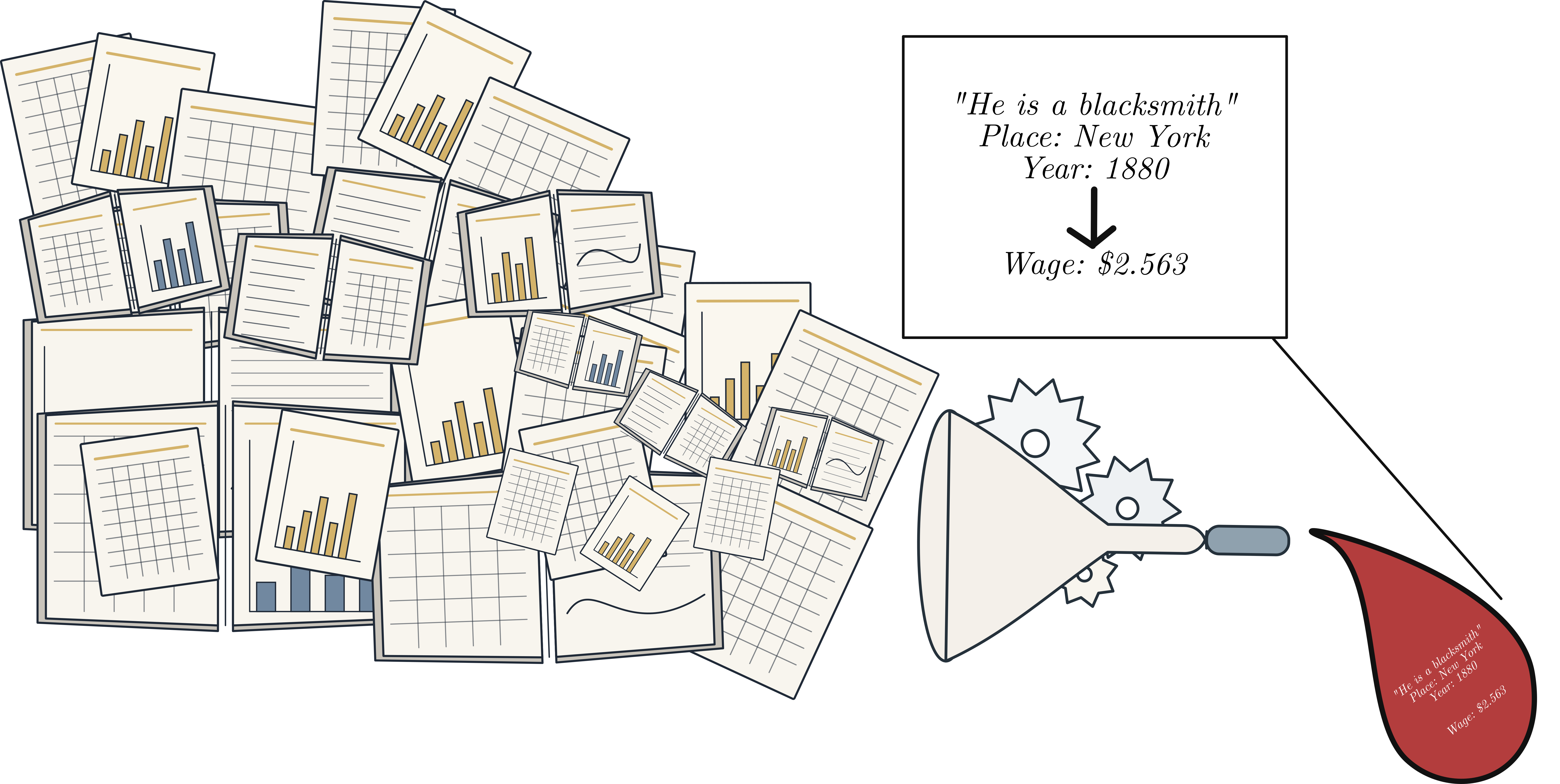

---
![CHAOS funnel](Figures/CHAOS_funnel1.png)

---
![CHAOS funnel](Figures/CHAOS_funnel2.png)

---
![CHAOS funnel](Figures/CHAOS_funnel3.png)

---
![CHAOS funnel](Figures/CHAOS_funnel4.png)

---
class: middle
# Broader reflection: Where are we going? (1/2)
.pull-left-wide[
- We need to validate, not just take ML predictions at face value. 
- We care more about bias than accuracy.
- Natural solution: 
  1. **Need for interpretable tools for Economic History**
  2. **It is fine to use black boxes if we can *debias* them.** (DSL, PPI, etc.)

]

.pull-right-narrow[
.small123[
*From Koschnick, Johansen, and Vedel (2026, unpublished)*
]
]

---
# Broader reflection: Why we use specific tools? (2/2)
.pull-left-wide[
.center[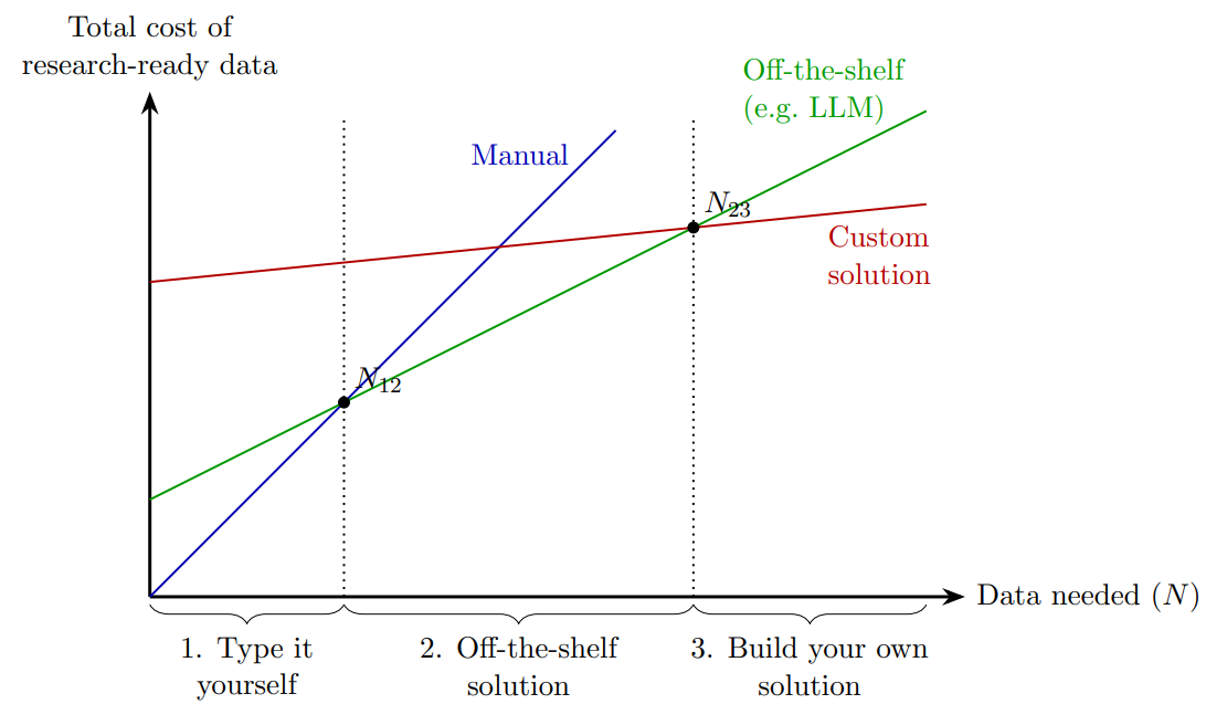![Cost](Figures/cost_ml_in_eh.png)]
]

.pull-right-narrow[
.small123[
*From Koschnick, Johansen, and Vedel (2026, unpublished)*
]
]

---
# The tool we present: *CHAOS*

1. If you have a *Source* containing: Occupations + some outcome (skills, income, etc.)

2. A *Target* containing: Occupations only (e.g. census data)

3. We provide a method for map any target occupation to a predicted outcome

**Approach:** Training a machine learning model on this is not generally feasible.

.chaosred[**We cheat:**] Turn probabilistic classifier into estimated regression function `$d\rightarrow \hat{y}$`.

.pull-left-narrow[
### What you provide:
- Source: `$\{d_i, y_i\}$`

| Occupation | Income |
|---|---|
| blacksmith | $2.30 |
| tailor | $1.98 |
| farmer | $1.42 |
]

.pull-right-wide[
.pull-left[
.large123[
  .chaosred[**CHAOS**]
  `$$\Rightarrow$$`
]
`$$\hat{y}(d) = \sum_{k} \hat{\mu}_k\, h(d, k)$$`
  
]

.pull-right[
### What you get:
- Target: `$\{d_k, \hat{y}_k\}$`

| Occupation | Income |
|---|---|
| smith | [Estimate] |
| tailor | [Estimate] |
| agricultural worker | [Estimate] |
]
]

---
name: literature

# Literature

.small123[
- IPUMS occscore introduced by Sobek (1995), but similar measures used throughout the literature (e.g. Preston & Haines 1991)

- This and similar measures have become prevalent in the literature.

- However, they entail a number of problems, mainly stemming from source-target-shift (Inwood et al. 2019, Saavedra & Twinam, 2020).

- A few fixes and alternative methods proposed (Saavedra & Twinam, 2020, Paker, Stephenson & Wallis, 2025, Vafa et al 2024, Mühlbach, 2021)

]

> .chaosred[**We propose a new method that is efficient and ML-powered but interpretable.**]

---
class: inverse, middle, center

# Econometric framework

---
name: bias

# Problem: Bias from occ. scores

`$$y_i = \alpha + \beta x_i + \varepsilon_i$$`

.small123[
where `$y_i$` is the true outcome (e.g. wage) to be replaced with `$\mu_S(d_i)$` s.t.
]

`$$\mu_S(d_i) = \alpha + \beta x_i + \varepsilon_i$$`

.pull-left-wide[
.small123[
Let `$\mu_S(d_i)$` be the source-assigned score, `$\mu_T(d_i)$` the target-population mean, `$y_i$` the true outcome. The total proxy error decomposes as:

`$$m_i \;=\; \underbrace{\mu_S(d_i) - \mu_T(d_i)}_{\delta(d_i)\ \text{source-target drift}} \;+\; \underbrace{\mu_T(d_i) - y_i}_{r_i\ \text{within-occupation residual}}$$`

Then:

`$$\hat{\beta} = \beta + \frac{\text{Cov}(x_i,\, m_i)}{\text{Var}(x_i)}$$`

]
]

.pull-right-narrow[
### The two big problems of occupational scores:
.small123[
`$\delta(d_i)$` — **source-target drift**
1950 US wages `$\neq$` 1850 England.

`$r_i$` — **within-occupation residual**
Apprentice `$\neq$` master;
]
]

.pull-left-wide[
`$$\require{cancel}$$`
`$m_i \;=\; \cancel{\underbrace{\mu_S(d_i) - \mu_T(d_i)}_{\delta(d_i)\ \text{source-target drift}}} \;+\; \underbrace{\mu_T(d_i) - y_i}_{r_i\ \text{within-occupation residual}}$`
]

.pull-right-narrow[
.chaosred[**CHAOS addresses the first and formalizes the second.**]
]

???

IPUMS occscore uses 1950 US wages --> Canadian migrants. Blacksmith rank shifts. Inwood et al. (2019).

r_i: "Smith" = goldsmith or blacksmith. "Tailor" = master or journeyman.

---
name: occcanine

# OccCANINE: the classifier

.pull-left[
.small123[w. Christian Møller Dahl & Torben Johansen — [arxiv 2402.13604](https://arxiv.org/abs/2402.13604)]

- Language model trained on **~18.5 million** observations
- 13 languages, 29 sources
- Open source, fast, highly accurate

**Key output:**

`$$\text{OccCANINE}: \quad d_i \;\mapsto\; \Pr(h_j \mid d_i)$$`

A full probability distribution over HISCO codes for any occupation string.

- Handles ambiguous, multi-occupation, and historical spelling

]

.pull-right[
![Architecture](Figures/Architecture_small.png)
.small123[*Conceptual architecture of OccCANINE*]
]

---
name: chaos-math

# The CHAOS estimator

1. **Source–target relevance** — source and target drawn from the same `$(D, Y, H)$` distribution
2. **Broadband** — `$\mathbb{E}[Y \mid H, D] = \mathbb{E}[Y \mid H]$`; the category is sufficient for `$Y$`
3. **Oracle access** — classifier gives `$h(d,k) = \Pr(H{=}k \mid D{=}d)$` for every description

.pull-left[
**Step A.1** — estimate (wrong) means from the source:

`$$\hat{r}_k = \frac{\sum_{i \in \mathcal{S}} Y_i\,h(D_i,k)}{\sum_{i \in \mathcal{S}} h(D_i,k)}$$`

This is biased, but we can get a handle on it:

`$$r_k = \sum_{j} A_{kj}\,\mu_j, \qquad A_{kj} = \mathbb{E}[h(D,j) \mid H=k]$$`

**Step A.2** — recover unbiased estimates by inverting the confusion matrix:

`$$\hat{\mu} = \hat{A}^{-1}\hat{r}$$`

]

.pull-right[
**Step B** — apply to any target description `$d$`:

`$$\hat{y}(d) = \sum_{k \in \mathcal{H}} \hat{\mu}_k\, h(d, k)$$`

Equivalently: `$\hat{y}(d) = \sum_{i \in \mathcal{S}} W_i(d)\,Y_i$` — a weighted average of source outcomes, with weights summing to 1.
]

[Why the correction is needed](#appendix-broadband-assumption)

---
name: method-check

# Checking results — evidence for each prediction

.pull-left[
### Evidence — how much of the source is about `$d$`?

`$$\widehat{\mathrm{ev}}(d) = \sum_{k} h(d,k)\;\frac{1}{n_{\mathcal{S}}}\sum_{i \in \mathcal{S}} h(D_i, k)$$`

> Share of the source truly belonging to this occupation. Computable from descriptions alone — before any outcome is collected.
]

.pull-right[
### Effective observations

`$$n_\text{eff}(d) = \frac{1}{\displaystyle\sum_i W_i(d)^2}$$`

> *How many source observations effectively back this prediction?*

- Accounts for the **confusion discount** — mass spread across HISCO codes reduces precision
- Equals `$N_\text{source} \times \text{Evidence}(d)$` only under hard assignment (`$A = I$`)
- Low `$n_\text{eff}$` `$\Rightarrow$` reverts toward the source mean
]

---
name: chaos-se

# Standard errors

.pull-left-wide[
> All sampling variation in `$\hat{y}(d)$` runs through a single residual `$\hat{\varepsilon}_i = Y_i - \hat{y}(D_i)$`.

.small123[*We can use this to build an influence function following Kennedy (2023)*]

]

.pull-left[
**Influence value** for observation `$i$` at target description `$d$`:

`$$\hat{\phi}_{d,i} = h(d)^\top \hat{A}^{-1}\hat{s}_i, \qquad \hat{s}_{i,k} = \frac{h(D_i,k)\;\hat{\varepsilon}_i}{\hat{B}_k}$$`

where `$\hat{B}_k = \frac{1}{n_\mathcal{S}}\sum_i h(D_i,k)$` is the average classifier mass on code `$k$`.
]

.pull-right[
**Standard error:**

`$$\widehat{\mathrm{se}}\bigl(\hat{y}(d)\bigr) = \sqrt{\frac{1}{n_{\mathcal{S}}^2}\sum_{i \in \mathcal{S}} \hat{\phi}_{d,i}^2}$$`

- One score per source row, no distributional assumptions
- Matches Monte Carlo standard deviations closely
]

[Full 3-step derivation](#appendix-influence-function)

---
class: inverse, middle, center

# Data and validation CHAOS predictions

---
name: application-data

# Source A — Wages (US Commissioner of Labor)

.pull-left-wide[
- **84,000 occupation–place–year** wage observations
- 140 places (US states + countries), 1725–1900
- Analysis sample (1800–1900): **135,182 obs**, 67 places, 4,492 occupations
- `$\Rightarrow$` Provides `$y_i$` (daily wages)

| Region | Obs | Places | Occupations |
|---|---|---|---|
| United States | 92,647 | 49 | 4,002 |
| United Kingdom | 18,793 | 5 | 1,617 |
| Western Europe | 23,742 | 13 | 2,002 |

- All of it digitized with Gemini and cleaned by hand
- **We supplement this with skills for 229 occupations from the London Tradesman (1747).** [See appendix](#appendix-source-b)
]

.pull-right-narrow[
.panelset[
.panel[.panel-name[Cover]
![COL cover](Figures/col-cover.png)
]
.panel[.panel-name[Table]
![COL table](Figures/col-first-tab.png)
]
]
]
---
name: chaos-flexibility

# CHAOS as a bridge between sources

.pull-right-wide[
.center[<img src="Figures/CHAOS_flexibility.png" width="100%">]
]

.pull-left-wide[
- Works in **any direction**
- In this application: **LTM skills (1747) `$\Rightarrow$` HISCO `$\Rightarrow$` DoL wages**
- In a nutshell: This gives intuition for the broadband classifier assumption — the HISCO layer is the "pivot" that allows us to connect different sources and time periods.
- *How much do you believe in HISCO? - Could use other classification systems.*
]

---
# Demonstration

.pull-left-narrow[

- This is all wrapped in a nice little python library.

]

.pull-right-wide[
  <iframe width="560" height="315" src="https://www.youtube.com/embed/WHCYSQp6yCk?si=lcKyQfj_3ZUYiRih" title="YouTube video player" frameborder="0" allow="accelerometer; autoplay; clipboard-write; encrypted-media; gyroscope; picture-in-picture; web-share" referrerpolicy="strict-origin-when-cross-origin" allowfullscreen></iframe>
  <br>
  [Short demonstration on YouTube](https://youtu.be/WHCYSQp6yCk)
  *Old version* - if time we will do live demo with the new version
]

---
# Validation exercise

*We run CHAOS on 1880 and try to predict 1860–1900 to showcase Source-Target drift.*

.pull-left-narrow[
- We have actual wages for 1860–1900
- So we can check how well CHAOS does in each year.
]

.pull-right-wide[

.panelset[
.panel[.panel-name[1881]
.center[<img src="Figures/validation_scatter_by_year/1881.png" width="100%">]
]
.panel[.panel-name[1882]
.center[<img src="Figures/validation_scatter_by_year/1882.png" width="100%">]
]
.panel[.panel-name[1883]
.center[<img src="Figures/validation_scatter_by_year/1883.png" width="100%">]
]
.panel[.panel-name[1894]
.center[<img src="Figures/validation_scatter_by_year/1894.png" width="100%">]
]
.panel[.panel-name[Bias]
.center[<img src="Figures/validation_prediction_error_histogram.png" width="100%">]
]
.panel[.panel-name[R^2]
.center[<img src="Figures/validation_rsq_by_year.png" width="100%">]
]
.panel[.panel-name[Wages]
.center[<img src="Figures/validation_raw_wages_by_year.png" width="100%">]
]
.panel[.panel-name[1895 base]
.center[<img src="Figures/validation_rsq_by_year_1895_baseline.png" width="100%">]
]
.panel[.panel-name[1894 rebased]
.center[<img src="Figures/validation_scatter_by_year_1895_baseline/1894.png" width="100%">]
]
.panel[.panel-name[Bias by year]
.center[<img src="Figures/validation_prediction_error_histogram_by_year.png" width="100%">]
]
]
]

---
name: method-check-traceability

# No black box — full traceability

.pull-left-narrow[
> Every prediction is a readable weighted average over source rows.

- Trace which HISCO codes contribute
- See the exact source occupations and weights
- Nothing hidden

]

.pull-right-wide[
.panelset[
.panel[.panel-name[Baker]
.center[<img src="Figures/sankey/he_is_a_baker.png" width="90%">]
]
.panel[.panel-name[Blacksmith]
.center[<img src="Figures/sankey/he_is_a_blacksmith.png" width="90%">]
]
.panel[.panel-name[Tailor]
.center[<img src="Figures/sankey/he_is_a_tailor.png" width="90%">]
]
.panel[.panel-name[Merchant]
.center[<img src="Figures/sankey/he_is_a_merchant.png" width="90%">]
]
]
]

[Appendix: step-by-step worked example](#appendix-blacksmith-example)

---
class: inverse, middle, center

# Application

---
name: applied-rq
class: middle

.pull-left-wide[
# Applied question

> What skills survive when the world turns upside down? The Industrial Revolution is our experiment — **skills locked in 1747**, outcomes traced across **regions, time, and gender**.

.small123[135,182 wage obs &middot; 67 places &middot; 1800–1900]

]

---
name: regression-setup

# Setup

.pull-left-wide[
.chaosred[**Warning:** Everything that follows is proof of concept. Do not believe anything you see.]

OLS throughout; SEs clustered by occupation. Skills from a **2×2 task framework**:

**Two continuous margins:**
- Routine vs. non-routine
- Cognitive vs. manual

**Four binary quadrant indicators** (mutually exclusive):
- Routine cognitive, non-routine cognitive, routine manual, non-routine manual
]

---
name: regression-specs

# Regression specifications

.pull-left-wide[

**Skill premium over time** — estimated separately per skill `$s$` and region `$r$`, reference 1800:
`$$\log w_{irt} = \sum_{t \neq 1800} \beta_t \bigl(s_i \cdot \mathbf{1}[\text{decade}=t]\bigr) + \gamma_t + \varepsilon_{irt}$$`

]

.pull-right-narrow[
- `$\gamma_t$` = decade fixed effects
- Run separately per skill and region
- **Continuous:** routine margin, cognitive margin
- **Binary:** 2×2 quadrant membership
- Weighted by CHAOS target evidence
]

---
name: skill-premiums-time

# Skill premiums over time, by region

.pull-left-narrow[
Coefficient = change in skill premium relative to 1800.

.chaosred[**Still preliminary**]

- No balancing
- No control for selection
- Just descriptive
]

.pull-right-wide[
.panelset[
.panel[.panel-name[Routine margin]
.center[<img src="Figures/time_region/weighted_routine_nonroutine_margin.png" width="85%">]
]
.panel[.panel-name[Cognitive margin]
.center[<img src="Figures/time_region/weighted_cognitive_noncognitive_margin.png" width="85%">]
]
.panel[.panel-name[Routine cognitive]
.center[<img src="Figures/time_region/weighted_is_routine_cognitive.png" width="85%">]
]
.panel[.panel-name[Non-routine cognitive]
.center[<img src="Figures/time_region/weighted_is_non_routine_cognitive.png" width="85%">]
]
.panel[.panel-name[Routine manual]
.center[<img src="Figures/time_region/weighted_is_routine_manual.png" width="85%">]
]
.panel[.panel-name[Non-routine manual]
.center[<img src="Figures/time_region/weighted_is_non_routine_manual.png" width="85%">]
]
]
]

---
name: conclusion

# Conclusion

.pull-left[
### Contributions

- **CHAOS:** probabilistic occupation scoring with confusion correction (`$\hat{A}^{-1}$`), standard errors via influence function, and full traceability
- **Empirical:** skill premiums across the industrializing world, 1800–1900 .chaosred[(preliminary)]

### What remains
- Validation against alternatives (OCCSCORE, HISCAM, HISCLASS), robustness, and extensions

**Email:** [christian-vs@sam.sdu.dk](mailto:christian-vs@sam.sdu.dk)
**BlueSky:** [@christianvedel.bsky.social](https://bsky.app/profile/christianvedel.bsky.social)
]

.pull-right[
![CHAOS pipeline](Figures/CHAOS.png)
]

---
class: middle, center, inverse

# Appendix

---
name: appendix-math-advanced

# CHAOS: multiple sources + debiasing .chaosred[(if time)]

.pull-left[
.small123[
### Multiple sources
When sources `$\mathcal{S}_1, \dots, \mathcal{S}_S$` are available, pool them to estimate `$\hat{A}$` and `$\hat{r}$`:

`$$\hat{A}_{kj} = \frac{\sum_s \sum_{i \in \mathcal{S}_s} h(D_i,j)\,h(D_i,k)}{\sum_s \sum_{i \in \mathcal{S}_s} h(D_i,k)}$$`

Then apply `$\hat{\mu} = \hat{A}^{-1}\hat{r}$` as before. No change to Step B.

### Gibberish input
If the classifier is uninformative: `$h(d,k) \approx \bar{h}_k$` (flat), then `$\hat{y}(d) \approx \bar{Y}$` — prediction reverts to the source mean.
]
]

.pull-right[
.small123[
### LOO calibration check

The `$\hat{A}^{-1}$` confusion correction ([see appendix](#appendix-confusion-correction)) supersedes the PPI-style mean correction.

A closed-form LOO residual provides a free calibration diagnostic — no extra computation needed:

`$$\hat{y}^{(-i)}(D_i) = \frac{\hat{y}(D_i) - P_{ii}\,Y_i}{1 - P_{ii}}$$`

where `$P_{ii} = h(D_i)^\top(\mathbf{H}^\top\mathbf{H})^{-1}h(D_i)$` is the hat-matrix leverage. If LOO predictions track source actuals, the `$\hat{A}^{-1}$` step is working.
]
]

[Back to slides](#motivation)

---
name: appendix-broadband-assumption

# Broadband — what the assumption really requires

> **Assumption 2 (Broadband):** `$\mathbb{E}[Y \mid H, D] = \mathbb{E}[Y \mid H]$`
> Once the occupational category is known, the text description adds no further information about the conditional mean of `$Y$`.

.pull-left-wide[
### Two conditions that satisfy it

1. **Hard assignment** — the classifier returns one code with probability 1. Knowing `$D$` already determines `$H$` exactly; the text carries no residual information.

2. **Constant within-category mean** — every description mapping to category `$k$` yields the same expected outcome, regardless of exact wording.

Classical scores (e.g. OCCSCORE) implicitly assume **(1)**. Probabilistic classifiers require making this explicit.
]

.pull-right-narrow[
.small123[
If a "journeyman blacksmith" and a "master blacksmith" earn different wages within HISCO 83110, neither condition holds — the Broadband assumption fails.

`$H$` must be sufficient for the regression of `$Y$` on `$(D, H)$`.
]
]

[Back to slides](#chaos-math)

---
name: appendix-confusion-bias

# The naive weighted average is biased

The natural first move — relevance-weighted average of source outcomes:

`$$\hat{r}_k = \frac{\sum_{i \in \mathcal{S}} Y_i \, h(D_i, k)}{\sum_{i \in \mathcal{S}} h(D_i, k)}$$`

.pull-left[
### What it converges to

`$$r_k = \sum_{j} A_{kj} \, \mu_j, \qquad A_{kj} = \mathbb{E}[h(D,j) \mid H = k]$$`

`$A_{kj}$` = expected classifier probability of category `$j$` among true-$k$ observations — the **confusion matrix**.

`$\hat{r}_k \to r_k \neq \mu_k$`
]

.pull-right[
### Intuition

| | `$h(\cdot, \text{blksmth})$` | `$h(\cdot, \text{hmrsmth})$` |
|---|---|---|
| "Blacksmith" | 0.955 | 0.011 |
| "Hammersmith" | **0.112** | 0.851 |

The blacksmith average absorbs hammersmith income. `$\hat{r}_\text{blacksmith}$` is dragged toward `$\mu_\text{hammersmith}$`.

.small123[Classical scores assume `$A = I$` — this contamination simply does not appear.]
]

[Back to slides](#chaos-math)

---
name: appendix-confusion-correction

# The fix: invert the confusion matrix

Since `$r = A\mu$` and `$A$` is identifiable from classifier probabilities alone, the correction is:

`$$\hat{\mu} = \hat{A}^{-1} \hat{r}$$`

.pull-left[
**Estimating `$\hat{A}$`** — no outcome data needed:

`$$\hat{A}_{kj} = \frac{\sum_{i \in \mathcal{S}} h(D_i, j)\, h(D_i, k)}{\sum_{i \in \mathcal{S}} h(D_i, k)}$$`

- Classical scores: `$A = I$` (implicit assumption)
- Sharp classifier: `$A \approx I$`, small correction
- Near-singular `$A$`: aggregate sibling codes
]

.pull-right[
**OLS equivalence** — `$\hat{\mu}$` is numerically identical to:

`$$\hat{\mu} = (\mathbf{H}^\top \mathbf{H})^{-1} \mathbf{H}^\top \mathbf{Y}$$`

No-intercept regression of `$Y_i$` on the probability vector `$h(D_i)$`.

]

[Back to slides](#chaos-math)

---
name: appendix-influence-function

# Standard errors via the influence function

Since `$h$` is known, all sampling variation comes from estimating `$(r, A)$` on `$\mathcal{S}$`.

.panelset[
.panel[.panel-name[Step 1: scores of r̂ and Â]

Both `$\hat{r}_k$` and `$\hat{A}_{kj}$` are ratios of sample means. The ratio rule for influence functions gives:

.pull-left[
`$$\phi^r_k(Y,D) = \frac{h(D,k)}{B_k}\bigl(Y - r_k\bigr)$$`
]

.pull-right[
`$$\phi^A_{kj}(D) = \frac{h(D,k)}{B_k}\bigl(h(D,j) - A_{kj}\bigr)$$`
]

where `$B_k = \mathbb{E}[h(D,k)]$` is the expected classifier mass on code `$k$`. The second follows from the first by replacing `$Y$` with `$h(D,j)$`.
]

.panel[.panel-name[Step 2: chain rule through Â⁻¹]

Perturbing `$\mu = A^{-1}r$` gives `$\mathrm{d}\mu = A^{-1}\bigl(\mathrm{d}r - (\mathrm{d}A)\mu\bigr)$`. The `$k$`-th entry of the bracket collapses:

.pull-left[
`$$\bigl(\phi^r - \phi^A\mu\bigr)_k = \frac{h(D,k)}{B_k}\,\varepsilon, \quad \varepsilon := Y - \mathbb{E}[Y \mid D]$$`

The entire influence function runs through a single residual `$\varepsilon$` — one score per source row, regardless of `$K$`.
]

.pull-right[
Compact form:

`$$\phi^\mu(Y,D) = A^{-1}\, s(Y,D), \quad s_k := \frac{h(D,k)\,\varepsilon}{B_k}$$`

The `$\hat{A}^{-1}$` correction propagates through the IF automatically.
]
]

.panel[.panel-name[Step 3: prediction SE]

For a fixed target description `$d$`, the IF of `$\hat{y}(d) = h(d)^\top\hat{\mu}$` is `$\phi_d = h(d)^\top A^{-1} s(Y,D)$`.

.pull-left[
Plug-in with `$(\hat{A},\hat{B},\hat{\mu})$` and residual `$\hat\varepsilon_i = Y_i - h(D_i)^\top\hat{\mu}$`:

`$$\hat{\phi}_{d,i} = h(d)^\top \hat{A}^{-1}\hat{s}_i, \quad \hat{s}_{i,k} = \frac{h(D_i,k)\,\hat\varepsilon_i}{\hat{B}_k}$$`
]

.pull-right[
Standard error from the sample variance of influence values:

`$$\widehat{\mathrm{se}}\bigl(\hat{y}(d)\bigr) = \sqrt{\frac{1}{n_{\mathcal{S}}^2}\sum_{i \in \mathcal{S}} \hat{\phi}_{d,i}^2}$$`

- One value per source row, no distributional assumptions
- Matches the simulation's Monte Carlo SDs closely
]
]
]

[Back to slides](#method-check)

---
name: appendix-blacksmith-example

# Worked example: "He is a blacksmith" (New York, 1880)

.panelset[
.panel[.panel-name[Source + classifier]

.pull-left[
Source `$\mathcal{S}$` — five wage observations:

| Title `$D_i$` | Wage `$Y_i$` |
|---|---|
| "Blacksmith" | \$2.80 |
| "Hammersmith" | \$2.55 |
| "Tinsmith" | \$2.30 |
| "Goldsmith" | \$3.10 |
| "Shoemaker" | \$2.40 |
]

.pull-right[
.small123[
OccCANINE probabilities `$h(D_i, k)$` — top 5 HISCO codes:

| | 83110 | 83120 | 87340 | 88050 | 80110 |
|---|---|---|---|---|---|
| Blacksmith | .955 | .011 | .018 | .013 | .003 |
| Hammersmith | **.112** | .851 | .031 | .000 | .006 |
| Tinsmith | .069 | .000 | .911 | .018 | .002 |
| Goldsmith | .074 | .011 | .012 | .901 | .002 |
| Shoemaker | .011 | .000 | .012 | .000 | .977 |

Codes: 83110 Blacksmith · 83120 Hammersmith · 87340 Tinsmith · 88050 Goldsmith · 80110 Shoemaker.  "Hammersmith" leaks 0.112 onto the blacksmith code.
]
]
]

.panel[.panel-name[Step A: correction]

.pull-left[
.small123[
HISCO-level estimates — top 5 codes:

| | 83110 | 83120 | 87340 | 88050 | 80110 |
|---|---|---|---|---|---|
| Mass `$s_k$` | 1.221 | 0.873 | 0.984 | 0.932 | 0.990 |
| Naive `$\hat{r}_k$` | 2.763 | 2.560 | 2.328 | 3.080 | 2.403 |
| CHAOS `$\hat{\mu}_k$` | **2.810** | 2.528 | 2.244 | 3.144 | 2.397 |
]
]

.pull-right[
`$\hat{r}_{83110} = 2.763$` sits **below** the observed \$2.80 — hammersmith contamination pulled it down.

After `$\hat{A}^{-1}$` correction: `$\hat{\mu}_{83110} = 2.810$` — recovered.

Diagonal of `$\hat{A}$` runs 0.77–0.96. Classical scores implicitly assume it equals 1.
]
]

.panel[.panel-name[Step B: prediction]

Target "He is a blacksmith" `$\;\Rightarrow\;$` `$h(d) = (0.951,\, 0.024,\, 0.013,\, 0.007,\, 0.005)$` `$\;\Rightarrow\;$` `$\hat{y}(d) = \mathbf{2.796}$`

.pull-left-wide[
.small123[
`$$\hat{y}(d) = 0.995 \times \underbrace{2.80}_\text{Blacksmith} + 0.015 \times \underbrace{2.55}_\text{Hammersmith} - 0.006 \times \underbrace{2.30}_\text{Tinsmith} - 0.006 \times \underbrace{3.10}_\text{Goldsmith} + 0.002 \times \underbrace{2.40}_\text{Shoemaker}$$`
]
]

.pull-right-narrow[
- Nearly all weight on the direct source
- Positive weight on the related hammersmith
- **Negative weights** subtract confusion contamination
- Weights sum to 1; `$n_\text{eff} \approx 1.0$`
]
]
]

[Back to slides](#method-check-traceability)

---
name: appendix-skills-ltm

# Skills from the London Tradesman (1747)

.pull-left-wide[
### Extracting skills
- GPT-4o returns a JSON list of skills per occupation from LTM descriptions

### Measuring skills (embedding distance)
- Map skill list `$S = \{s_1, \dots, s_N\}$` into 384-dim space via Sentence-BERT (all-MiniLM-L6-v2)
- Construct skill index via cosine similarity to anchor phrases:

`$$\text{routine proportion}_i = \frac{\bar{\sigma}_{i,\text{routine}}}{\bar{\sigma}_{i,\text{routine}} + \bar{\sigma}_{i,\text{non-routine}}}$$`
]

.pull-right-narrow[
.panelset[
.panel[.panel-name[Goldsmith skills]
.tiny123[
`"making all manner of utensils in gold or silver"`,
`"casting works with raised figures in moulds"`,
`"polishing and finishing cast works"`,
`"using flatting-mills to reduce metal to required thinness"`,
`"making all moulds for their work"`
]
]
.panel[.panel-name[Anchors]
.small123[
**Routine:** repetitive task, following explicit rules, highly structured sequence

**Cognitive:** abstract reasoning, analytical thinking, information processing

**Mechanical:** operate machinery, assemble parts, machine operation
]
]
]
]

[Back to slides](#application-data)

---
name: appendix-ny

# Sankey examples — input text to estimated wage

.panelset[
.panel[.panel-name[Baker]
.center[<img src="Figures/sankey/he_is_a_baker.png" width="72%">]
]
.panel[.panel-name[Blacksmith]
.center[<img src="Figures/sankey/he_is_a_blacksmith.png" width="72%">]
]
.panel[.panel-name[Tailor]
.center[<img src="Figures/sankey/he_is_a_tailor.png" width="72%">]
]
.panel[.panel-name[Carpenter]
.center[<img src="Figures/sankey/he_works_as_a_carpenter.png" width="72%">]
]
.panel[.panel-name[Merchant]
.center[<img src="Figures/sankey/he_is_a_merchant.png" width="72%">]
]
.panel[.panel-name[Physician]
.center[<img src="Figures/sankey/he_is_a_physician.png" width="72%">]
]
.panel[.panel-name[Miner]
.center[<img src="Figures/sankey/he_is_a_miner.png" width="72%">]
]
]

[Back to slides](#method-check-traceability)

---
name: appendix-bias-rhs

# Bias when the occupational score is on the RHS

.pull-left-wide[
Now suppose `$\hat{y}_i$` is the **explanatory variable**:

`$$x_i = \alpha + \beta_2 \hat{y}_i + \varepsilon_i, \quad \hat{y}_i = y_i + m_i$$`

The OLS estimator gives:

`$$\hat{\beta}_2 = \beta_2 \!\left(1 - \frac{\text{Var}(m_i)}{\text{Var}(y_i)}
\right) - \frac{\text{Cov}(y_i,\, m_i)}{\text{Var}(y_i)} + \frac{\text{Cov}(m_i,\, \varepsilon_i)}{\text{Var}(y_i)}$$`

Two sources of bias:

1. **Attenuation** -- `$\text{Var}(m_i)$` dilutes the signal, shrinking `$\hat{\beta}_2$` toward zero
2. **Correlation bias** -- if `$m_i$` co-moves with `$y_i$` or `$\varepsilon_i$`, slope shifts unpredictably
]

.pull-right-narrow[
Recall `$m_i = \hat{y}_i - y_i$` decomposes as `$\delta(d_i) + r_i$` (drift + residual):

- `$\delta$` correlated with `$x_i$` `$\Rightarrow$` correlation bias. CHAOS .green[**reduces**] `$\delta$`.
- `$r_i$` correlated with `$x_i$` `$\Rightarrow$` .chaosred[**irreducible.**]
- Attenuation always present; CHAOS reduces `$\text{Var}(m_i)$` by eliminating `$\delta$`.
]

---
name: appendix-source-b

# Source B — Skills (London Tradesman, 1747)

.pull-left-wide[
- 229 occupations with natural-language skill descriptions from Campbell (1747)

**Four-step pipeline:**
1. **LLM (GPT-4o)** extracts structured skill list per occupation
2. **Sentence-BERT** embeds skills; cosine similarity to anchor phrases gives `$\text{Score}(c) = \max_{s \in S}\,\text{score}(s,c)$`
3. **Discrete classification** — max rule maps scores to mutually exclusive categories: routine/non-routine × cognitive/manual (+ mechanical dimension)
4. **CHAOS** maps occupation-level scores to HISCO-level indices
]

.pull-right-narrow[
.panelset[
.panel[.panel-name[Book]
![LTM](Figures/ltm.png)
]
.panel[.panel-name[Example]
![LTM example](Figures/ltm_example.png)
]
.panel[.panel-name[Semantic space]

![Skills in semantic space](Figures/skills_illustration.png)
]
]
]

[Skills measurement details](#appendix-skills-ltm)

[Back to slides](#application-data)

---
name: appendix-wages-premia

# Wages and skill premia

.panelset[
.panel[.panel-name[Wages NY over time]
.center[<img src="Figures/wages_ny_over_time.png" width="90%">]
]
.panel[.panel-name[Skill premia USA]
.center[<img src="Figures/skill_premia_over_time_usa.png" width="90%">]
]
]

---
name: appendix-2d-task-space

# Occupations in 2D task space

.center[<img src="Figures/occupations_2d_matrix_simple_top2_zoom_labeled.png" width="60%">]

[Back to slides](#regression-setup)

---
name: appendix-category-aggregation

# When `$\hat{A}$` is near-singular: aggregate sibling codes

If the condition number `$\kappa(\hat{A}) > \tau$`, matrix inversion amplifies noise. The fix: coarsen the code space by merging hard-to-separate codes.

.pull-left[
### Greedy algorithm

1. Compute SVD of `$\hat{A}$`; if `$\kappa \leq \tau$`, stop
2. Find `$k^* = \arg\max_k |v_{K',k}|$` — the code most loaded on the smallest singular direction
3. Collapse all siblings of `$k^*$` to their parent in the HISCO hierarchy; update `$\hat{A}$` and `$\hat{r}$` in `$O(K'^2)$`
4. Repeat until `$\kappa \leq \tau$`
]

.pull-right[
### Trade-off

- **Fine codes** `$\Rightarrow$` sharper category means, but `$\hat{A}$` risks near-singularity
- **Coarse codes** `$\Rightarrow$` stable `$\hat{A}$`, but category means are pooled
- Aggregation introduces bias only if merged codes have genuinely different true means
- `$\tau = 30$` in practice; typically reduces the active code set by `$\sim 10\times$`
]

[Back to slides](#appendix-confusion-correction)

---
name: appendix-references

# References

.tiny123[
.pull-left[
Sobek, Matthew (1995). "The Comparability of Occupations and the Generation of Income Scores." *Historical Methods* 28(1): 47–51.

Inwood, Kris, Chris Minns, and Fraser Summerfield (2019). "Occupational Income Scores and Immigrant Assimilation: Evidence from the Canadian Census." *Explorations in Economic History* 72: 114–122.

Saavedra, Martin, and Tomas Twinam (2020). "A Machine Learning Approach to Improving Occupational Income Scores." *Explorations in Economic History* 75: 101304.

Dahl, Christian Møller, Torben Johansen, and Christian Vedel (2024). "Breaking the HISCO Barrier: Automatic Occupational Standardization with OccCANINE." arXiv:2402.13604.

Vafa, Keyon, Emil Palikot, Tian Du, Ayush Kanodia, Susan Athey, and David M. Blei (2024). "CAREER: A Foundation Model for Labor Sequence Data." arXiv:2202.08370.

Goldin, Claudia, and Lawrence F. Katz (1998). "The Origins of Technology-Skill Complementarity." *Quarterly Journal of Economics* 113(3): 693–732.

Autor, David H., Frank Levy, and Richard J. Murnane (2003). "The Skill Content of Recent Technological Change: An Empirical Exploration." *Quarterly Journal of Economics* 118(4): 1279–1333.

Acemoglu, Daron, and David Autor (2011). "Skills, Tasks and Technologies: Implications for Employment and Earnings." In *Handbook of Labor Economics*, Vol. 4B, pp. 1043–1171.

Franck, Raphael, and Oded Galor (2022). "Technology-Skill Complementarity in the Early Phase of Industrialization." *Economic Journal* 132(642): 618–643.

Kogan, Leonid, Dimitris Papanikolaou, Lawrence D. W. Schmidt, and Bryan Seegmiller (2021). "Technology, Vintage-Specific Human Capital, and Labor Displacement." *NBER Working Paper* 29552.

Atack, Jeremy, Robert A. Margo, and Paul W. Rhode (2022). "Mechanization Takes Command?" *Journal of Economic History* 82(3): 663–689.

Autor, David H., David Dorn, and Gordon H. Hanson (2013). "The China Syndrome." *American Economic Review* 103(6): 2121–2168.

Autor, David H., David Dorn, and Gordon H. Hanson (2016). "The China Shock." *Annual Review of Economics* 8: 205–240.

Acemoglu, Daron, and Pascual Restrepo (2019). "Automation and New Tasks." *Journal of Economic Perspectives* 33(2): 3–30.

Acemoglu, Daron, and Pascual Restrepo (2020). "Robots and Jobs." *Journal of Political Economy* 128(6): 2188–2244.
]

.pull-right[
McCloskey, Deirdre N. (2010). *Bourgeois Dignity*. Chicago: University of Chicago Press.

Allen, Robert C. (2009). *The British Industrial Revolution in Global Perspective*. Cambridge: Cambridge University Press.

Clark, Gregory (2007). *A Farewell to Alms*. Princeton: Princeton University Press.

Mokyr, Joel (2009). *The Enlightened Economy*. New Haven: Yale University Press.

Squicciarini, Mara P., and Nico Voigtländer (2015). "Human Capital and Industrialization: Evidence from the Age of Enlightenment." *Quarterly Journal of Economics* 130(4): 1825–1883.

Feldman, Naomi E., and Karine van der Beek (2016). "Skill Choice and Skill Complementarity in Eighteenth Century England." *Explorations in Economic History* 59: 94–113.

de Pleijt, Alexandra, Alessandro Nuvolari, and Jacob Weisdorf (2020). "Human Capital Formation during the First Industrial Revolution." *Journal of the European Economic Association* 18(2): 829–889.

Cinnirella, Francesco, Erik Hornung, and Julius Koschnick (2025). "Flow of Ideas: Economic Societies and the Rise of Useful Knowledge." *Economic Journal* 135(669): 1496–1535.

de Pleijt, Alexandra, Julius Koschnick, and Patrick Wallis (2026). "Education and Skills during the First Industrial Revolution in England." *LSE Economic History Working Paper* 393.

Angelopoulos, Anastasios N., Stephen Bates, Clara Fannjiang, Michael I. Jordan, and Tijana Zrnic (2023). "Prediction-Powered Inference." *Science* 382(6671): 669–674.

Ludwig, Jens, Sendhil Mullainathan, and Ashesh Rambachan (2025). "Large Language Models: An Applied Econometric Framework." *NBER Working Paper* 33344.

Bound, John, Charles Brown, and Nancy Mathiowetz (2001). "Measurement Error in Survey Data." In *Handbook of Econometrics*, Vol. 5, pp. 3705–3843.

Kennedy, Edward H. (2023). "Semiparametric Doubly Robust Targeted Double Machine Learning: A Review." arXiv:2203.06469.

Hampole, Menaka, Dimitris Papanikolaou, Lawrence D. W. Schmidt, and Bryan Seegmiller (2025). "Artificial Intelligence and the Labor Market." *NBER Working Paper*.
]
]